An Introduction to Automatic Differentiation

The chain rule is all you need: an introduction to mathematical foundations of automatic differentiation.

Motivation

To apply gradient-based optimization methods such as stochastic gradient descent to a neural network, we need to compute the gradient of its loss function with respect to its parameters.

Since deep learning models can get large and complicated, it would be nice to have machinery that can take an arbitrary function $f: \mathbb{R}^{n} \rightarrow \mathbb{R}^{m}$ and return its derivative. This is called automatic differentiation (AD).

The Julia AD ecosystem

Julia has more than a dozen AD systems. A summary of available packages can be found at juliadiff.org. The list is sorted by type:

Reverse-mode
Forward-mode
Symbolic
Finite differencing

and other more exotic approaches. These are already abstract sounding terms, but within these categories, there are further differences:

Is the AD system operator overloading or source-to-source?
Which representation level does it operate on?
Does it only work on scalar functions?
Does it allow higher-order AD?

As you may not be familiar with these terms, the goal of this lecture is to explain differences in approaches between various AD packages and outline their pros and cons.

For this purpose, we will take a step back and start with a recapitulation of two fundamental mathematical concepts: linear maps and derivatives.

Linear maps

Properties

Linear maps, also called linear transformations, are functions with the following properties:

Property	Equation	property satisfied¹	property not satisfied¹
Additivity	$f(v_1+v_2) = f(v_1) + f(v_2)$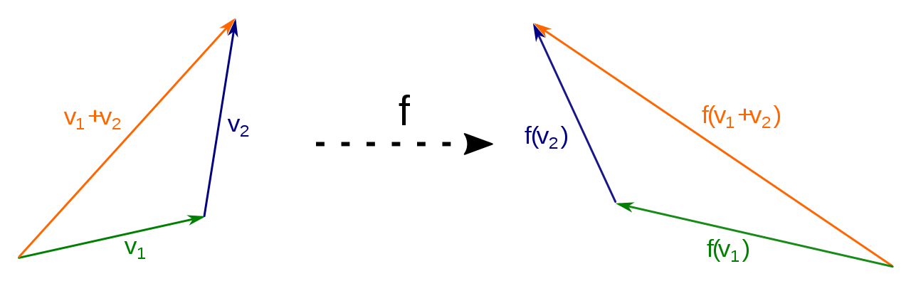
Homogeneity	$f(\lambda v) = \lambda f(v)$

Visualizations by Stephan Kulla, CC0.

Mathematically more rigorous definition:

Assuming two arbitrary vector spaces $V, W$ over the field $K$, a function $f:V\rightarrow W$ is called a linear map if additivity and homogeneity are satisfied for any vectors $v_1, v_2 \in V$ and $\lambda \in K$.

Connection to matrices

Every linear map $f$ between two finite-dimensional vector spaces $V, W$ can be represented as a matrix, given a basis for each vector space (e.g. the standard basis).

A linear map $f: \mathbb{R}^{n} \rightarrow \mathbb{R}^{m}$ can be represented as

$$ f(x) = Ax $$

where $A$ is a $m \times n$ matrix and $x \in \mathbb{R}^{n}$.

Example

Linear maps $f: \mathbb{R}^2 \rightarrow \mathbb{R}^2$ can be represented as $2 \times 2$ matrices.

Many common geometric transformations are linear maps, for example

Transformation	Matrix representation
Rotations by angle $\theta$	$\begin{pmatrix} \cos\theta & -\sin\theta \\ \sin\theta & \cos\theta \end{pmatrix}$
Projection on $y$-axis	$\begin{pmatrix} 0 & 0 \\ 0 & 1 \end{pmatrix}$
Reflection through $y$-axis	$\begin{pmatrix} -1 & 0 \\ 0 & 1 \end{pmatrix}$
Stretching along $y$-axis	$\begin{pmatrix} 1 & 0 \\ 0 & k \end{pmatrix}$
Shearing parallel to $y$-axis	$\begin{pmatrix} 1 & 0 \\ k & 1 \end{pmatrix}$
Squeezing	$\begin{pmatrix} k & 0 \\ 0 & \frac{1}{k} \end{pmatrix}$

for the basis $e_x = (1, 0)$, $e_y = (0, 1)$.

Composition

Connection to matrix multiplication

The composition $h(x) = g(f(x))$ of two linear maps $f: V \rightarrow W$, $g: W \rightarrow Z$ is also a linear map $h: V \rightarrow Z$.

In finite-dimensional vector spaces, the composition of linear maps corresponds to matrix multiplication:

$$ \begin{aligned} f(x) &= Fx &, \enspace &f: \mathbb{R}^{m} \rightarrow \mathbb{R}^{n} &, \enspace &F \in \mathbb{R}^{n \times m} \\ g(x) &= Gx &, \enspace &g: \mathbb{R}^{n} \rightarrow \mathbb{R}^{p} &, \enspace &G \in \mathbb{R}^{p \times n} \\ h(x) = (g \circ f)(x) &= (G \cdot F) x = Hx &, \enspace &h: \mathbb{R}^{m} \rightarrow \mathbb{R}^{p} &, \enspace &H \in \mathbb{R}^{p \times m} \\ \end{aligned} $$

Connection to matrix addition

The sum of two linear maps $f_1: V \rightarrow W$, $f_2: V \rightarrow W$ is also a linear map:

$(f_1 + f_2)(x) = f_1(x) + f_2(x) \quad$

In finite-dimensional vector spaces, the addition of linear maps corresponds to matrix addition.

For $f_1$ and $f_2: \mathbb{R}^{n} \rightarrow \mathbb{R}^{m}$ and $A, B \in \mathbb{R}^{m \times n}$

$$ \begin{aligned} f_1(x) &= Ax \\ f_2(x) &= Bx \\ (f_1 + f_2)(x) &= (A+B)x \quad . \end{aligned} $$

Derivatives

What is a derivative?

The (total) derivative of a function $f: \mathbb{R}^{n} \rightarrow \mathbb{R}^{m}$ at a point $\tilde{x} \in \mathbb{R}^{n}$ is the linear approximation of $f$ near the point $\tilde{x}$.

We give the derivative the symbol $\mathcal{D}f_{\tilde{x}}$. You can read this as "$\mathcal{D}$erivative of $f$ at $\tilde{x}$".

Most importantly, the derivative is a linear map

$$ \mathcal{D}f_{\tilde{x}}: \mathbb{R}^{n} \rightarrow \mathbb{R}^{m} \quad . $$

Let's visualize this on a simple scalar function:

$$ f(x) = x^2 - 5 \sin(x) - 10 $$

Plot showing the function f(x) = x² - 5sin(x) - 10 in blue, its derivative as an orange line through the origin, and the first-order Taylor approximation in green tangent to f at the expansion point.

The orange line $\mathcal{D}f_{\tilde{x}}$ is of biggest interest to us. Notice how the derivative fulfills homogeneity: it always goes through the origin $(x,y)=(0,0).$

Using $\mathcal{D}f_{\tilde{x}}$, we can construct the first order Taylor series approximation of $f$ around $\tilde{x}$ (shown in green). For points close to $\tilde{x},$

$$ f(x) \approx f(\tilde{x}) + \mathcal{D}f_{\tilde{x}}(x-\tilde{x}) \quad . $$

Differentiability

From your calculus classes, you might recall that a function $f: \mathbb{R} \rightarrow \mathbb{R}$ is differentiable at $\tilde{x}$ if there is a number $f'(\tilde{x})$ such that

$$ \lim_{h \rightarrow 0} \frac{f(\tilde{x} + h) - f(\tilde{x})}{h} = f'(\tilde{x}) \quad . $$

This number $f'(\tilde{x})$ is called the derivative of $f$ at $\tilde{x}$.

We can now extend this notion to multivariate functions: A function $f: \mathbb{R}^{n} \rightarrow \mathbb{R}^{m}$ is totally differentiable at a point $\tilde{x}$ if there exists a linear map $\mathcal{D}f_{\tilde{x}}$ such that

$$ \lim_{h \rightarrow 0} \frac{|f(\tilde{x} + h) - f(\tilde{x}) - \mathcal{D}f_{\tilde{x}}(h)|}{|h|} = 0 \quad . $$

Jacobians

Linear maps $f: \mathbb{R}^{n} \rightarrow \mathbb{R}^{m}$ can be represented as a $m \times n$ matrices.

In the standard basis, the matrix corresponding to $\mathcal{D}f$ is called the Jacobian:

$$ J_f = \begin{bmatrix} \dfrac{\partial f_1}{\partial x_1} & \cdots & \dfrac{\partial f_1}{\partial x_n}\\ \vdots & \ddots & \vdots\\ \dfrac{\partial f_m}{\partial x_1} & \cdots & \dfrac{\partial f_m}{\partial x_n} \end{bmatrix} $$

Note that every entry $[J_f]_{ij}=\frac{\partial f_i}{\partial x_j}$ in this matrix is a scalar function $\mathbb{R} \rightarrow \mathbb{R}$.

If we evaluate the Jacobian at a specific point $\tilde{x}$, we get the matrix corresponding to $\mathcal{D}f_{\tilde{x}}$:

$$ J_f\big|_{\tilde{x}} = \begin{bmatrix} \dfrac{\partial f_1}{\partial x_1}\Bigg|_{\tilde{x}} & \cdots & \dfrac{\partial f_1}{\partial x_n}\Bigg|_{\tilde{x}}\\ \vdots & \ddots & \vdots\\ \dfrac{\partial f_m}{\partial x_1}\Bigg|_{\tilde{x}} & \cdots & \dfrac{\partial f_m}{\partial x_n}\Bigg|_{\tilde{x}} \end{bmatrix} \in \mathbb{R}^{m \times n} $$

Example

Given the function $f: \mathbb{R}^2 \rightarrow \mathbb{R}^2$

$$ f\left(\begin{bmatrix} x_1\\x_2\end{bmatrix}\right) = \begin{bmatrix} x_1^2 x_2 \\5 x_1 + \sin x_2 \end{bmatrix} \quad , $$

we obtain the $2 \times 2,$ Jacobian

$$ J_f = \begin{bmatrix} \dfrac{\partial f_1}{\partial x_1} & \dfrac{\partial f_1}{\partial x_2} \\ \dfrac{\partial f_2}{\partial x_1} & \dfrac{\partial f_2}{\partial x_2} \end{bmatrix} = \begin{bmatrix} 2 x_1 x_2 & x_1^2 \\ 5 & \cos x_2 \end{bmatrix} \quad . $$

At the point $\tilde{x} = (2, 0)$, the Jacobian is

$$ J_f\big|_{\tilde{x}} = \begin{bmatrix} 0 & 4 \\ 5 & 1 \end{bmatrix} \quad . $$

In the standard basis, our linear map $\mathcal{D}f_{\tilde{x}}: \mathbb{R}^2 \rightarrow \mathbb{R}^2$ therefore corresponds to

$$ \mathcal{D}f_{\tilde{x}}(v) = J_f\big|_{\tilde{x}} \cdot v = \begin{bmatrix} 0 & 4 \\ 5 & 1 \end{bmatrix} \begin{bmatrix} v_1 \\ v_2 \end{bmatrix} \quad , $$

for some input vector $v \in \mathbb{R}^2$.

Jacobian-Vector products

As we have seen in the example above, the total derivative²

$$ \mathcal{D}f_{\tilde{x}}(v) = J_f\big|_{\tilde{x}} \cdot v $$

computes a Jacobian-Vector product. It is also called the "pushforward" and is one of the two core primitives behind AD systems:

Jacobian-Vector products (JVPs) computed by the pushforward, used in forward-mode AD
Vector-Jacobian products (VJPs) computed by the pullback, used in reverse-mode AD

In our notation, all vectors $v$ are column vectors and row vectors are written as $v^T$.

Chain rule

Let's look at a function $h(x)=g(f(x))$ composed from two differentiable functions

$f: \mathbb{R}^{n} \rightarrow \mathbb{R}^{m}$ and $g: \mathbb{R}^{m} \rightarrow \mathbb{R}^{p} $:

$$ h = g \circ f, . $$

Since derivatives are linear maps, we can obtain the derivate of $h$ by composing the derivatives of $g$ and $f$ using the chain rule:

$$ \mathcal{D}h_{\tilde{x}} = \mathcal{D}(g \circ f)_{\tilde{x}} = \mathcal{D}g_{f(\tilde{x})} \circ \mathcal{D}f_{\tilde{x}} $$

As we have seen in the section on linear maps, this composition of linear maps is also a linear map. It corresponds to simple matrix multiplication.³

A proof of the chain rule can be found on page 19 of Spivak's Calculus on Manifolds.

Example

We just introduced a form of the chain rule that works on arbitrary input and output dimensions $n$, $m$ and $p$. Let's show that we can recover the product rule

$$ (uv)' = u'v+uv' $$

of two scalar functions $u(t)$, $v(t)$. We start out by defining

$$ g(u, v) = u \cdot v \qquad f(t) = \begin{bmatrix} u(t) \\ v(t) \end{bmatrix} $$

such that

$$ h(t) = (g \circ f)(t) = u(t) \cdot v(t) \quad . $$

The derivatives of $f$ and $g,$ are

$$ \mathcal{D}g = \begin{bmatrix} \frac{\partial g}{\partial u} & \frac{\partial g}{\partial v} \end{bmatrix} = \begin{bmatrix} v & u \end{bmatrix} $$

$$ \mathcal{D}f = \begin{bmatrix} \frac{\partial f_1}{\partial t} \\ \frac{\partial f_2}{\partial t} \end{bmatrix} = \begin{bmatrix} u' \\ v' \end{bmatrix} $$

Using the chain rule, we can compose these derivatives to obtain the derivative of $h$:

$$ \begin{aligned} (uv)' = \mathcal{D}h &= \mathcal{D}(g \circ f) \\ &= \mathcal{D}g \circ \mathcal{D}f \\ &= \begin{bmatrix} v & u \end{bmatrix} \cdot \begin{bmatrix} u' \\ v' \end{bmatrix} \\ &= vu' + uv' \end{aligned} $$

As you can see, the product rule follows from the chain rule. Instead of memorizing several different rules, the chain rule reduces everything to the composition of linear maps, which corresponds to matrix multiplication.